MINF3650

(30 pts) Create a basic Excel worksheet

Review the Excel 101 video.
Create an Excel worksheet named Budget.xslx which meets the following specifications and layout
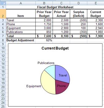
1. Prior Year Budget and Prior Year Actual columns and the Budget Adjustment (percent in Cell B8) are plugged numbers; all other value cells should be derived using formulas.
2. Surplus(Deficit) is calculated as Prior Year Budget – Prior Year Actual.
3. Current Budget is calculated as Prior Year Budget – Budget Adjustment * Surplus(Deficit) and the formula should use an absolute reference to Budget Adjustment.
4. The Total row contains simple column totals.
5. The pie chart should appear with the spreadsheet and show how the Current Budget is divided among the budget components.
6. Formatting similar to that in the screen shot and a 'pleasing' placement of charts is expected.
In addition to the example data, add a row for Entertainment with Prior Year Budget equal to $1000 plus the last 3 digits of your 927 number and Prior Year Actual equal to $2000 minus the last 3 digits of your 927 number. Spreadsheet totals and the pie chart should include these data.
Beyond the video: Revise the formula for Current Budget from 2.3 above so that when Surplus(Deficit) is negative (i.e., a deficit) only half the Budget Adjustment percentage is applied. Hint: Lookup help on the Excel IF function and use Budget Adjustment / 2 as the multiplier when Surplus(Deficit) < 0.
Beyond the video: In addition to the pie chart include a column chart which shows three columns for each budget item: Prior Year Budget, Prior Year Actual, Current Budget. Place the column chart below or to the right of the pie chart. Hint: Use help on column charts in Excel.
Save the completed Budget.xslx and Submit through your MIS lab.

(20 pts) Practice with introductory Excel pivot tables

Review the Excel Pivot Tables video which focuses on this particular example.
Download and use the AdventureWorksCustomers spreadsheet as a starting point; it shows AdventureWorks customers attributes including whether they have purchased a bicycle.
In the following inquiries be sure pivot table clearly shows the answer to the query question:
1. Add a tab named EdOcc which analyzes the percentage of AdventureWorks customers who purchased bicycles for every combination of Education and Occupation.
2. Add a tab named IncAnaly which provides the average income for every combination of Marital Status & Gender.
3. Add a tab named AvgAge which provides the average age of customers who purchased bicycles.
4. Beyond the video: Add a tab named ChildrenAndCars show the average and standard deviation of income for every combination of Children and Cars.
5. Beyond the video: Add a tab named OccReg which shows a count of customers for each Occupation and Region.
Save the completed spreadsheet and submit through MIS lab.